We start by importing the required libraries.
import matplotlib.pyplot as plt
import json
import numpy as np
import os
import tensorflow as tf
import tensorflow.keras.layers as tfl

from tensorflow.keras.preprocessing import image_dataset_from_directory
from tensorflow.keras.layers.experimental.preprocessing import RandomFlip, RandomRotation
Creating a Dataset
When training and evaluating deep learning model in Keras, generating a dataset from image files stored on disk is simple and fast.
BATCH_SIZE = 32
IMG_SIZE = (160, 160)
directory = "dataset/"
train_dataset = image_dataset_from_directory(directory,
                                             shuffle = True,
                                             batch_size = BATCH_SIZE,
                                             image_size = IMG_SIZE,
                                             validation_split = 0.2,
                                             subset = 'training',
                                             seed = 42)

validation_dataset = image_dataset_from_directory(directory,
                                             shuffle=True,
                                             batch_size=BATCH_SIZE,
                                             image_size=IMG_SIZE,
                                             validation_split=0.2,
                                             subset='validation',
                                             seed=42)
Preprocess and Augmentation
We use prefetch() to prevent a memory bottleneck that can occur when reading from disk. This method sets aside some data and keeps it ready for when needed, by creating a source dataset from our input data, applying a transformation to preprocess it, then iterating over the dataset one element at a time. Because the iteration is streaming, the data does not need to fit into memory.
We can set the number of elements to prefetch manually, or we could use tf.data.experimental.AUTOTUNE to choose the parameters automatically. Autotune prompts tf.data to tune that value dynamically at runtime, by tracking the time spent in each operation and feeding those times into an optimization algorithm. The optimization algorithm tries to find the best allocation of its CPU budget across all tunable operations.
AUTOTUNE = tf.data.experimental.AUTOTUNE
train_dataset = train_dataset.prefetch(buffer_size=AUTOTUNE)
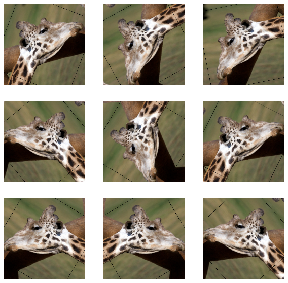
To increase diversity in the training set and help our model learn better, we augment the images by transforming them.
def data_augmenter():
    '''
    Create a Sequential model composed of 2 layers
    Returns:
        tf.keras.Sequential
    '''
    data_augmentation = tf.keras.Sequential()
    data_augmentation.add(RandomFlip("horizontal"))
    data_augmentation.add(RandomRotation(0.2))

    return data_augmentation
Now we use this function to transform our data.
data_augmentation = data_augmenter()

for image, _ in train_dataset.take(1):
    plt.figure(figsize=(10, 10))
    first_image = image[0]
    for i in range(9):
        ax = plt.subplot(3, 3, i + 1)
        augmented_image = data_augmentation(tf.expand_dims(first_image, 0))
        plt.imshow(augmented_image[0] / 255)
        plt.axis('off')
This give output :
Since we are using a pre-trained model that was trained on the normalization value , it is best practice to reuse that standard with tf.keras.applications.mobilenet_v2.preprocess_input.
preprocess_input = tf.keras.applications.mobilenet_v2.preprocess_inputUsing MobileNetV2 for Transfer Learning
MobileNetV2 was trained on ImageNet and is optimized to run on mobile and other low-power applications. It’s 155 layers deep and very efficient for object detection and image segmentation tasks, as well as classification tasks like this one. The architecture has three defining characteristics:
- Depthwise separable convolutions
- Thin input and output bottlenecks between layers
- Shortcut connections between bottleneck layers
Now we will set how we can use the pre-trained model to modify the classifier task so that it is able to recognize alpacas.
def alpaca_model(image_shape=IMG_SIZE, data_augmentation=data_augmenter()):
    ''' Define a tf.keras model for binary classification out of the MobileNetV2 model
    Arguments:
        image_shape -- Image width and height
        data_augmentation -- data augmentation function
    Returns:
    Returns:
        tf.keras.model
    '''


    input_shape = image_shape + (3,)
     base_model_path="imagenet_base_model/without_top_mobilenet_v2_weights_tf_dim_ordering_tf_kernels_1.0_160_no_top.h5"

    base_model = tf.keras.applications.MobileNetV2(input_shape= input_shape,
                                                   include_top= False,
                                                   weights=base_model_path)

    # freeze the base model by making it non trainable
    base_model.trainable = False
    # create the input layer (Same as the imageNetv2 input size)
    inputs = tf.keras.Input(shape=input_shape)
    x = data_augmentation(inputs)
    x = preprocess_input(x)
    x = base_model(x, training=False)

    # add the new Binary classification layers
    # use global avg pooling to summarize the info in each channel
    x = tf.keras.layers.GlobalAveragePooling2D()(x)
    # include dropout with probability of 0.2 to avoid overfitting
    x = tf.keras.layers.Dropout(0.2)(x)

    # use a prediction layer with one neuron (as a binary classifier only needs one)
    outputs = tf.keras.layers.Dense(1)(x)

    model = tf.keras.Model(inputs, outputs)
    return model
We now define the model,
model2 = alpaca_model(IMG_SIZE, data_augmentation)Now let us train the model.
base_learning_rate = 0.001
model2.compile(optimizer=tf.keras.optimizers.Adam(lr=base_learning_rate),
              loss=tf.keras.losses.BinaryCrossentropy(from_logits=True),
              metrics=['accuracy'])
initial_epochs = 5
history = model2.fit(train_dataset, validation_data=validation_dataset, epochs=initial_epochs)We get the following output :
Epoch 1/5
9/9 [==============================] - 9s 1s/step - loss: 0.7764 - accuracy: 0.5496 - val_loss: 0.6586 - val_accuracy: 0.5846

Epoch 2/5
9/9 [==============================] - 8s 857ms/step - loss: 0.7139 - accuracy: 0.5840 - val_loss: 0.5791 - val_accuracy: 0.6154

Epoch 3/5
9/9 [==============================] - 8s 835ms/step - loss: 0.5629 - accuracy: 0.6794 - val_loss: 0.4570 - val_accuracy: 0.7385

Epoch 4/5
9/9 [==============================] - 8s 846ms/step - loss: 0.4899 - accuracy: 0.7137 - val_loss: 0.4403 - val_accuracy: 0.6769

Epoch 5/5
9/9 [==============================] - 8s 846ms/step - loss: 0.4404 - accuracy: 0.7481 - val_loss: 0.3806 - val_accuracy: 0.7077
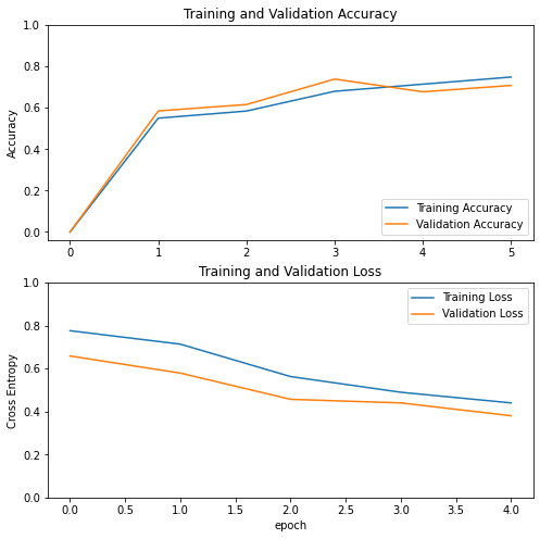
The results are okay, but could be better. Next we will try some fine-tuning on the model.
Fine-tuning the Model
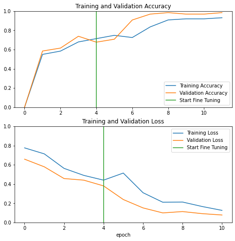
We can try fine-tuning the model by re-running the optimizer in the last layers to improve accuracy. In transfer learning, the way we can achieve this is by unfreezing the layers at the end of the network, and then re-training our model on the final layers with a very low learning rate.
The intuition for what’s happening: when the network is in its earlier stages, it trains on low-level features, like edges. In the later layers, more complex, high-level features like wispy hair or pointy ears begin to emerge. For transfer learning, the low-level features can be kept the same, as they have common features for most images. When we add new data, we generally want the high-level features to adapt to it, which is rather like letting the network learn to detect features more related to your data, such as soft fur or big teeth.
base_model = model2.layers[4]
base_model.trainable = True

# Fine-tune from this layer onwards
fine_tune_at = 120
# Freeze all the layers before the `fine_tune_at` layer
for layer in base_model.layers[:fine_tune_at]:
    layer.trainable = False

loss_function= tf.keras.losses.BinaryCrossentropy(from_logits = True)
optimizer = tf.keras.optimizers.Adam(lr = 0.1*base_learning_rate)
metrics=['accuracy']

model2.compile(loss=loss_function,
              optimizer = optimizer,
              metrics=metrics)
Now we fine tune
fine_tune_epochs = 5
total_epochs =  initial_epochs + fine_tune_epochs

history_fine = model2.fit(train_dataset,
                         epochs=total_epochs,
                         initial_epoch=history.epoch[-1],
                         validation_data=validation_dataset)
We get the following output :
Epoch 5/10
9/9 [==============================] - 10s 1s/step - loss: 0.5140 - accuracy: 0.7252 - val_loss: 0.2387 - val_accuracy: 0.9077

Epoch 6/10
9/9 [==============================] - 9s 1s/step - loss: 0.3094 - accuracy: 0.8359 - val_loss: 0.1513 - val_accuracy: 0.9692

Epoch 7/10
9/9 [==============================] - 9s 991ms/step - loss: 0.2104 - accuracy: 0.9084 - val_loss: 0.0993 - val_accuracy: 0.9846

Epoch 8/10
9/9 [==============================] - 9s 1s/step - loss: 0.2125 - accuracy: 0.9198 - val_loss: 0.1132 - val_accuracy: 0.9692

Epoch 9/10
9/9 [==============================] - 9s 1s/step - loss: 0.1656 - accuracy: 0.9198 - val_loss: 0.0915 - val_accuracy: 0.9692

Epoch 10/10
9/9 [==============================] - 9s 992ms/step - loss: 0.1256 - accuracy: 0.9313 - val_loss: 0.0773 - val_accuracy: 0.9846
What we should remember:
- To adapt the classifier to new data: Delete the top layer, add a new classification layer, and train only on that layer
- When freezing layers, avoid keeping track of statistics (like in the batch normalization layer)
- Fine-tune the final layers of your model to capture high-level details near the end of the network and potentially improve accuracy
Now that we have seen Classification in depth, let us look at Object Detection.