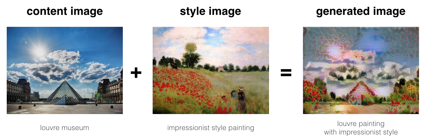
Code implementation of Neural Style Transfer

We will import the packages we want first.

import os
import sys
import scipy.io
import scipy.misc
import matplotlib.pyplot as plt
from matplotlib.pyplot import imshow
from PIL import Image
import numpy as np
import tensorflow as tf
import pprint
%matplotlib inline

Transfer Learning

Neural Style Transfer uses a previously trained convolutional network, and builds on top of that. We will be using the eponymously named VGG network. We will first load the model.

tf.random.set_seed(272) 
pp = pprint.PrettyPrinter(indent=4)
img_size = 400
vgg = tf.keras.applications.VGG19(include_top=False,
                                  input_shape=(img_size, img_size, 3),
                                  weights='pretrained-model/vgg19_weights_tf_dim_ordering_tf_kernels_notop.h5')
 
vgg.trainable = False

Neural Style Transfer

Next we will define the cost functions for content and style and later the overall cost function.

Computing Content Cost

content_image = Image.open("images/louvre.jpg")
print("The content image (C) shows the Louvre museum's pyramid surrounded by old Paris buildings, against a sunny sky with a few clouds.")
content_image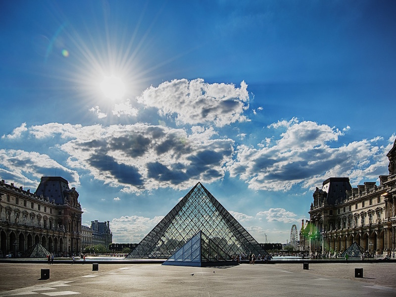

We want to calculate the cost :

J_{co n t e n t} (C, G) = \frac{1}{4 \times n _{H} \times n _{W} \times n _{C}} all entries \sum (a^{(C)} - a^{(G)})^{2} (1)

def compute_content_cost(content_output, generated_output):
    """
    Computes the content cost
    
    Arguments:
    a_C -- tensor of dimension (1, n_H, n_W, n_C), hidden layer activations representing content of the image C 
    a_G -- tensor of dimension (1, n_H, n_W, n_C), hidden layer activations representing content of the image G
    
    Returns: 
    J_content -- scalar that you compute using equation 1 above.
    """
    a_C = content_output[-1]
    a_G = generated_output[-1]
    
    _, n_H, n_W, n_C = a_G.get_shape().as_list()
    
    a_C_unrolled = tf.reshape(a_C, shape=[1, n_H * n_W, n_C])
    a_G_unrolled = tf.reshape(a_G, shape=[1, n_H * n_W, n_C])
    
    J_content = tf.reduce_sum(tf.square(tf.subtract(a_C_unrolled, a_G_unrolled)))/(4*n_H*n_C*n_W)
        
    return J_content

Computing Style Cost

Let us see an example of the style image.

example = Image.open("images/monet_800600.jpg")
example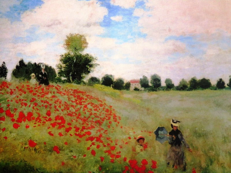

We first define the style matrix which is also known as the Gram matrix. In linear algebra, the Gram matrix G of a set of vectors $(v_{1}, \dots, v_{n})$ is the matrix of dot products, whose entries are $G_{ij} = v_{i}^{T} v_{j} = n p . d o t (v_{i}, v_{j})$ . In other words, $G_{ij}$ compares how similar $v_{i}$ is to $v_{j}$ : If they are highly similar, you would expect them to have a large dot product, and thus for $G_{ij}$ to be large.

G is also used to represent the generated image, so to represent the matrix we will use $G_{g r am}$ .

def gram_matrix(A):
    """
    Argument:
    A -- matrix of shape (n_C, n_H*n_W)
    
    Returns:
    GA -- Gram matrix of A, of shape (n_C, n_C)
    """  
    GA = tf.matmul(A, tf.transpose(A))
 
    return GA

Now that we can calculate the Gram matrix we can calculate the style cost.

For now, you will use only a single hidden layer $a^{[l]}$ .
The corresponding style cost for this layer is defined as:

J_{s t y l e}^{[l]} (S, G) = \frac{1}{4 \times n _{C} ^{2} \times ( n _{H} \times n _{W} ) ^{2}} i = 1 \sum n_{C} j = 1 \sum n_{C} (G_{(g r am) i, j}^{(S)} - G_{(g r am) i, j}^{(G)})^{2} (2)

$G_{g r am}^{(S)}$ Gram matrix of the “style” image.
$G_{g r am}^{(G)}$ Gram matrix of the “generated” image.
Cost is computed using the hidden layer activations for a particular hidden layer in the network $a^{[l]}$

def compute_layer_style_cost(a_S, a_G):
    """
    Arguments:
    a_S -- tensor of dimension (1, n_H, n_W, n_C), hidden layer activations representing style of the image S 
    a_G -- tensor of dimension (1, n_H, n_W, n_C), hidden layer activations representing style of the image G
    
    Returns: 
    J_style_layer -- tensor representing a scalar value, style cost defined above by equation (2)
    """
 
    _, n_H, n_W, n_C = a_G.get_shape().as_list()
    
    a_S = tf.transpose(tf.reshape(a_S, [n_H * n_W, n_C]))
    a_G = tf.transpose(tf.reshape(a_G, [n_H * n_W, n_C]))
 
    GS = gram_matrix(a_S)
    GG = gram_matrix(a_G)
 
    J_style_layer = tf.reduce_sum(tf.square(tf.subtract(GS, GG)))/(4*(n_C**2)*(n_H*n_W)**2)
        
    return J_style_layer

So far we have captures the style from only one layer. We get better results if we merge style cost from several different layers. Each layer will be given weights (𝜆[𝑙]) that reflect how much each layer will contribute to the style. Let us start listing the layer names :

for layer in vgg.layers:
   print(layer.name)

This gives output :

input_1
block1_conv1
block1_conv2
block1_pool
block2_conv1
block2_conv2
block2_pool
block3_conv1
block3_conv2
block3_conv3
block3_conv4
block3_pool
block4_conv1
block4_conv2
block4_conv3
block4_conv4
block4_pool
block5_conv1
block5_conv2
block5_conv3
block5_conv4
block5_pool

Now choose layers to represent the style of the image and assign style costs:

STYLE_LAYERS = [
    ('block1_conv1', 0.2),
    ('block2_conv1', 0.2),
    ('block3_conv1', 0.2),
    ('block4_conv1', 0.2),
    ('block5_conv1', 0.2)]

You can combine the style costs for different layers as follows:

J_{s t y l e} (S, G) = l \sum λ^{[l]} J_{s t y l e}^{[l]} (S, G)

where the values for $λ^{[l]}$ are given in STYLE_LAYERS.

def compute_style_cost(style_image_output, generated_image_output, STYLE_LAYERS=STYLE_LAYERS):
    """
    Computes the overall style cost from several chosen layers
    
    Arguments:
    style_image_output -- our tensorflow model
    generated_image_output --
    STYLE_LAYERS -- A python list containing:
                        - the names of the layers we would like to extract style from
                        - a coefficient for each of them
    
    Returns: 
    J_style -- tensor representing a scalar value, style cost defined above by equation (2)
    """
    
    J_style = 0
    a_S = style_image_output[:-1]
 
    a_G = generated_image_output[:-1]
    for i, weight in zip(range(len(a_S)), STYLE_LAYERS):  
        J_style_layer = compute_layer_style_cost(a_S[i], a_G[i])
        J_style += weight[1] * J_style_layer
 
    return J_style

Defining the Total Cost to Optimize

@tf.function()
def total_cost(J_content, J_style, alpha = 10, beta = 40):
    """
    Computes the total cost function
    
    Arguments:
    J_content -- content cost coded above
    J_style -- style cost coded above
    alpha -- hyperparameter weighting the importance of the content cost
    beta -- hyperparameter weighting the importance of the style cost
    
    Returns:
    J -- total cost as defined by the formula above.
    """
 
    J = alpha*J_content + beta*J_style
 
    return J

Now we will randomly initialize the image to be generated.

generated_image = tf.Variable(tf.image.convert_image_dtype(content_image, tf.float32))
noise = tf.random.uniform(tf.shape(generated_image), -0.25, 0.25)
generated_image = tf.add(generated_image, noise)
generated_image = tf.clip_by_value(generated_image, clip_value_min=0.0, clip_value_max=1.0)
 
print(generated_image.shape)
imshow(generated_image.numpy()[0])
plt.show()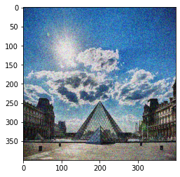

Training and Inference

def get_layer_outputs(vgg, layer_names):
    """ Creates a vgg model that returns a list of intermediate output values."""
    outputs = [vgg.get_layer(layer[0]).output for layer in layer_names]
 
    model = tf.keras.Model([vgg.input], outputs)
    return model

content_layer = [('block5_conv4', 1)]
 
vgg_model_outputs = get_layer_outputs(vgg, STYLE_LAYERS + content_layer)

content_target = vgg_model_outputs(content_image)  # Content encoder
style_targets = vgg_model_outputs(style_image)     # Style encoder

We have built the model, and now to compute the content cost, we will encode our content image using the appropriate hidden layer activations. Set this encoding to the variable a_C. Later we will need to do the same for the generated image, by setting the variable a_G to be the appropriate hidden layer activations. We will use layer block5_conv4 to compute the encoding. The code below does the following:

preprocessed_content =  tf.Variable(tf.image.convert_image_dtype(content_image, tf.float32))
a_C = vgg_model_outputs(preprocessed_content)
 
preprocessed_style =  tf.Variable(tf.image.convert_image_dtype(style_image, tf.float32))
a_S = vgg_model_outputs(preprocessed_style)

Below are the utils that you will need to display the images generated by the style transfer model.

def clip_0_1(image):
    """
    Truncate all the pixels in the tensor to be between 0 and 1
    
    Arguments:
    image -- Tensor
    J_style -- style cost coded above
 
    Returns:
    Tensor
    """
    return tf.clip_by_value(image, clip_value_min=0.0, clip_value_max=1.0)
 
def tensor_to_image(tensor):
    """
    Converts the given tensor into a PIL image
    
    Arguments:
    tensor -- Tensor
    
    Returns:
    Image: A PIL image
    """
    tensor = tensor * 255
    tensor = np.array(tensor, dtype=np.uint8)
    if np.ndim(tensor) > 3:
        assert tensor.shape[0] == 1
        tensor = tensor[0]
    return Image.fromarray(tensor)

Now we will train the transfer learning. We use Adam optimizer and learning rate of 0.01.

optimizer = tf.keras.optimizers.Adam(learning_rate=0.01)
 
@tf.function()
def train_step(generated_image):
    with tf.GradientTape() as tape:
        a_G = vgg_model_outputs(generated_image)
        J_style = compute_style_cost(a_S, a_G)
        J_content = compute_content_cost(a_C, a_G)
        J = total_cost(J_content, J_style)
        
    grad = tape.gradient(J, generated_image)
    optimizer.apply_gradients([(grad, generated_image)])
    generated_image.assign(clip_0_1(generated_image))
    return J

epochs = 2501
for i in range(epochs):
    train_step(generated_image)
    if i % 250 == 0:
        print(f"Epoch {i} ")
    if i % 250 == 0:
        image = tensor_to_image(generated_image)
        imshow(image)
        image.save(f"output/image_{i}.jpg")
        plt.show()

# Show the 3 images in a row
fig = plt.figure(figsize=(16, 4))
ax = fig.add_subplot(1, 3, 1)
imshow(content_image[0])
ax.title.set_text('Content image')
ax = fig.add_subplot(1, 3, 2)
imshow(style_image[0])
ax.title.set_text('Style image')
ax = fig.add_subplot(1, 3, 3)
imshow(generated_image[0])
ax.title.set_text('Generated image')
plt.show()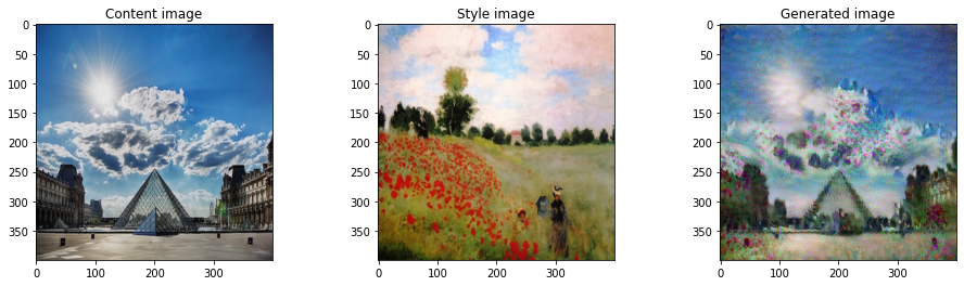

Running for around epochs = 20000 with a learning_rate=0.001 we get the following more improved output :

Digital Garden

Explorer