Code implementation of Residual Networks

We start by importing the required libraries.

import tensorflow as tf
import numpy as np
import scipy.misc
from tensorflow.keras.applications.resnet_v2 import ResNet50V2
from tensorflow.keras.preprocessing import image
from tensorflow.keras.applications.resnet_v2 import preprocess_input, decode_predictions
from tensorflow.keras import layers
from tensorflow.keras.layers import Input, Add, Dense, Activation, ZeroPadding2D, Flatten, Conv2D, AveragePooling2D, MaxPooling2D, GlobalMaxPooling2D
from tensorflow.keras.models import Model, load_model
from resnets_utils import *
from tensorflow.keras.initializers import random_uniform, glorot_uniform, constant, identity
from tensorflow.python.framework.ops import EagerTensor
from matplotlib.pyplot import imshow
 
%matplotlib.inline
np.random.seed(1)
tf.random.set_seed(2)

The problem of Very Deep Neural Networks

Neural networks in the recent recent years have become much deeper. The main benefit of very deep networks is that it can represent very complex functions. It can also learn features at many different levels of abstraction.

However, using a deeper network does not always help. A huge barrier to training them is the problem of vanishing and exploding gradients.

To solve this problem we use a Residual Network. in ResNets a skip connection allows the model to skip layers. This ‘skip connection’ makes it very easy for one of the blocks to learn an identity function.

Identity block

The identity block is the standard block used in ResNets and corresponds to the case where the input activation (say $a^{[l]}$) has the same dimension as the output activation (say $a^{[l+2]}$). These are the individual steps for a skip connection that “skips” over 2 layers :

• The first CONV2D has $F_1$ filters of shape (1, 1) and a stride of (1, 1).
• The first BatchNorm is normalizing the ‘channels’ axis.
• Then apply the ReLU activation function. This has no hyper-parameters.
• The second CONV2D has $F_2$ filters of shape (1, 1) and a stride of (1, 1).
• The second BatchNorm is normalizing the ‘channels’ axis.
• Here the ReLU function is not applied first. The X_shortcut and the output of the 2nd layer X are added together.
• Then we apply the ReLU function.

How we will implement a identity block for a skip connection that “skip over” 3 hidden layers rather than 2 layers.

def identity_block(X, f, filters, initializer=random_uniform):
    """
    Arguments:
    X -- input tensor of shape (m, n_H_prev, n_W_prev, n_C_prev)
    f -- integer, specifying the shape of the middle CONV's window for the main path
    filters -- python list of integers, defining the number of filters in the CONV layers of the main path
    initializer -- to set up the initial weights of a layer. Equals to random uniform initializer
    
    Returns:
    X -- output of the identity block, tensor of shape (m, n_H, n_W, n_C)
    """
    F1, F2, F3 = filters
    X_shortcut = X
    
    X = Conv2D(filters = F1, 
               kernel_size = 1, 
               strides = (1,1), 
               padding = 'valid', 
               kernel_initializer = initializer(seed=0))(X)
    X = BatchNormalization(axis = 3)(X) 
    X = Activation('relu')(X)
    
    X = Conv2D(filters=F2,
           kernel_size=(f, f),
           strides=(1,1),
           padding='same',
           kernel_initializer=initializer(seed=0))(X)
    X = BatchNormalization(axis=3)(X)
    X = Activation('relu')(X)
 
    X = Conv2D(filters=F3,
           kernel_size=(1,1),
           strides=(1,1),
           padding='valid',
           kernel_initializer=initializer(seed=0))(X)
    X = BatchNormalization(axis=3)(X)
 
    X = Add()([X, X_shortcut])
    X = Activation('relu')(X)
    
    return X

Convolution block

The ResNet “convolutional block” is the second block type. We use this block when the input and output dimensions do not match up. The difference with the identity block is that there is a CONV2D layer in the shortcut path. Here is how we can implement it :

def convolutional_block(X, f, filters, s = 2, initializer=glorot_uniform):
    """
    Arguments:
    X -- input tensor of shape (m, n_H_prev, n_W_prev, n_C_prev)
    f -- integer, specifying the shape of the middle CONV's window for the main path
    filters -- python list of integers, defining the number of filters in the CONV layers of the main path
    s -- Integer, specifying the stride to be used
    initializer -- to set up the initial weights of a layer. Equals to Glorot uniform initializer, 
                   also called Xavier uniform initializer.
    
    Returns:
    X -- output of the convolutional block, tensor of shape (m, n_H, n_W, n_C)
    """
    F1, F2, F3 = filters
    X_shortcut = X
 
    X = Conv2D(filters = F1, 
               kernel_size = 1, 
               strides = (s, s), 
               padding='valid', 
               kernel_initializer = initializer(seed=0))(X)
    X = BatchNormalization(axis = 3)(X)
    X = Activation('relu')(X)
 
    X = Conv2D(filters = F2, 
               kernel_size = (f, f), 
               strides = (1, 1), 
               padding='same', 
               kernel_initializer = initializer(seed=0))(X)
    X = BatchNormalization(axis = 3)(X)
    X = Activation('relu')(X)
 
    X = Conv2D(filters = F3, 
               kernel_size = 1, 
               strides = (1, 1), 
               padding='valid', 
               kernel_initializer = initializer(seed=0))(X)
    X = BatchNormalization(axis = 3)(X)
    
    X_shortcut = Conv2D(filters = F3, 
                 kernel_size = 1, 
                 strides = (s, s), 
                 padding='valid', 
                 kernel_initializer = initializer(seed=0))(X_shortcut)
    X_shortcut = BatchNormalization(axis = 3)(X_shortcut)
    
    X = Add()([X, X_shortcut])
    X = Activation('relu')(X)
    
    return X

Building a ResNet Model

We now have the necessary blocks to build a very deep ResNet. The following figure describes in detail the architecture of this neural network. “ID BLOCK” in the diagram stands for “Identity block,” and “ID BLOCK x3” means you should stack 3 identity blocks together.

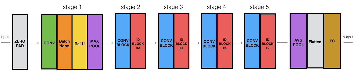
def ResNet50(input_shape = (64, 64, 3), classes = 6, training=False):
    """
    Stage-wise implementation of the architecture of the popular ResNet50:
    CONV2D -> BATCHNORM -> RELU -> MAXPOOL -> CONVBLOCK -> IDBLOCK*2 -> CONVBLOCK -> IDBLOCK*3
    -> CONVBLOCK -> IDBLOCK*5 -> CONVBLOCK -> IDBLOCK*2 -> AVGPOOL -> FLATTEN -> DENSE 
 
    Arguments:
    input_shape -- shape of the images of the dataset
    classes -- integer, number of classes
 
    Returns:
    model -- a Model() instance in Keras
    """
    
    X_input = Input(input_shape)
    X = ZeroPadding2D((3, 3))(X_input)
    
    X = Conv2D(64, (7, 7), 
               strides = (2, 2), 
               kernel_initializer = glorot_uniform(seed=0))(X)
    X = BatchNormalization(axis = 3)(X)
    X = Activation('relu')(X)
    X = MaxPooling2D((3, 3), strides=(2, 2))(X)
 
    X = convolutional_block(X, f = 3, filters = [64, 64, 256], s = 1)
    X = identity_block(X, 3, [64, 64, 256])
    X = identity_block(X, 3, [64, 64, 256])
 
    X = convolutional_block(X, f = 3, filters = [128,128,512], s = 2)
    X = identity_block(X, 3, [128,128,512])
    X = identity_block(X, 3, [128,128,512])
    X = identity_block(X, 3, [128,128,512])
 
    X = convolutional_block(X, f = 3, filters = [256, 256, 1024], s = 2)
    X = identity_block(X, 3, [256, 256, 1024])
    X = identity_block(X, 3, [256, 256, 1024])
    X = identity_block(X, 3, [256, 256, 1024])
    X = identity_block(X, 3, [256, 256, 1024])
    X = identity_block(X, 3, [256, 256, 1024])
 
    X = convolutional_block(X, f = 3, filters = [512, 512, 2048], s = 2)
    X = identity_block(X, 3, [512, 512, 2048])
    X = identity_block(X, 3, [512, 512, 2048])
 
    X = AveragePooling2D((2, 2), strides=(1, 1))(X)
    X = Flatten()(X)
    X = Dense(classes, 
              activation='softmax', 
              kernel_initializer = glorot_uniform(seed=0))(X)
    
    model = Model(inputs = X_input, outputs = X)
 
    return model

Now we will compile the model.

np.random.seed(1)
tf.random.set_seed(2)
opt = tf.keras.optimizers.Adam(learning_rate=0.00015)
model.compile(optimizer=opt, loss='categorical_crossentropy', metrics=['accuracy'])

The model is now ready to be trained. The only thing we need now is a dataset. We train the model on the SIGNS dataset.

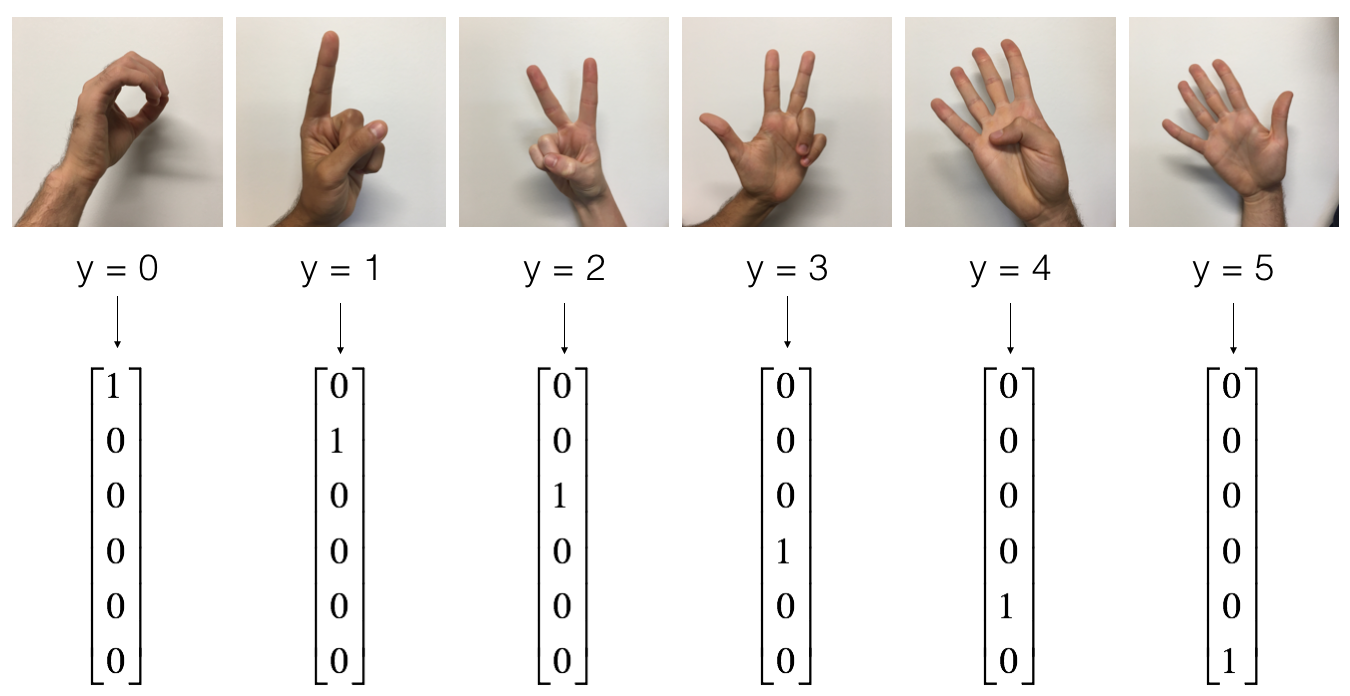
X_train_orig, Y_train_orig, X_test_orig, Y_test_orig, classes = load_dataset()
 
X_train = X_train_orig / 255.
X_test = X_test_orig / 255.
 
Y_train = convert_to_one_hot(Y_train_orig, 6).T
Y_test = convert_to_one_hot(Y_test_orig, 6).T
 
print ("number of training examples = " + str(X_train.shape[0]))
print ("number of test examples = " + str(X_test.shape[0]))
print ("X_train shape: " + str(X_train.shape))
print ("Y_train shape: " + str(Y_train.shape))
print ("X_test shape: " + str(X_test.shape))
print ("Y_test shape: " + str(Y_test.shape))

Output :

number of training examples = 1080
number of test examples = 120
X_train shape: (1080, 64, 64, 3)
Y_train shape: (1080, 6)
X_test shape: (120, 64, 64, 3)
Y_test shape: (120, 6)

We trained the model as follows.

model.fit(X_train, Y_train, epochs = 10, batch_size = 32)

Output :

Epoch 1/10
34/34 [==============================] - 11s 43ms/step - loss: 1.8407 - accuracy: 0.3241

Epoch 2/10
34/34 [==============================] - 1s 43ms/step - loss: 1.1585 - accuracy: 0.5481

Epoch 3/10
34/34 [==============================] - 1s 42ms/step - loss: 0.8954 - accuracy: 0.6648

Epoch 4/10
34/34 [==============================] - 1s 41ms/step - loss: 0.6625 - accuracy: 0.7593

Epoch 5/10
34/34 [==============================] - 1s 41ms/step - loss: 0.4561 - accuracy: 0.8398

Epoch 6/10
34/34 [==============================] - 1s 42ms/step - loss: 0.2727 - accuracy: 0.9028

Epoch 7/10
34/34 [==============================] - 1s 41ms/step - loss: 0.2396 - accuracy: 0.9130

Epoch 8/10
34/34 [==============================] - 1s 41ms/step - loss: 0.2236 - accuracy: 0.9176

Epoch 9/10
34/34 [==============================] - 1s 40ms/step - loss: 0.2433 - accuracy: 0.9157

Epoch 10/10
34/34 [==============================] - 1s 40ms/step - loss: 0.2135 - accuracy: 0.938

preds = model.evaluate(X_test, Y_test)
print ("Loss = " + str(preds[0]))
print ("Test Accuracy = " + str(preds[1]))

Output :

4/4 [==============================] - 1s 10ms/step - loss: 0.5922 - accuracy: 0.8000
Loss = 0.5922172665596008
Test Accuracy = 0.800000011920929

We get a test accuracy of 80 %. When train the complete ResNet50 on a GPU we achieve test accuracy to as close as 94 %.