Attention Is All You Need

Introduction

This paper introduces an alternative state of the art architecture called the Transformer. Previously recurrent neural networks, long short-term memory and gated recurrent neural networks had been used to approach sequence modeling.

Recurrent models compute a hidden state say $h_{t}$ , as a function of the previous state $h_{t - 1}$ and the input at that position $t$ . This inherently sequence natures precludes parallelization and also puts forwards memory constraints for longer sequences.

For more on sequence models you can refer to Sequence models.

Background

The goal of reducing sequential computation also forms the foundation of the Extended Neural GPU, ByteNet and ConvS2S, all of which use convolutional neural networks as basic building blocks and help in computing hidden states in parallel.

The problem with those CNN-based models: Even though they’re parallel, they still struggle to connect information between two positions that are far apart in the sequence. Think of a CNN layer as only “seeing” a small local window (its kernel size) at a time. To connect word 1 and word 100, you need to stack many layers so the “receptive field” grows enough to cover that distance.

For ConvS2S, the number of layers needed grows linearly with the distance between positions.
For ByteNet, it grows logarithmically (better, but still grows).

This matters because the more “hops” or operations needed to relate two distant positions, the harder it is for the model to learn dependencies between them — the signal has to pass through more transformations and can degrade.

How the Transformer fixes this: Self-attention lets any position directly attend to any other position in a single step — a constant number of operations, regardless of distance. Word 1 and word 100 are just as directly connected as word 1 and word 2.

This directness comes at a cost. When you attend to many positions at once, we compute weighted average of their representations. Averaging blurs things together, so we lose precision. To fix this we use Multi-Head Attention. Instead of doing one averaging operation, the model runs several attention “heads” in parallel, each learning to focus on different aspects/positions. This recovers the resolution lost from averaging, since different heads can specialize in different relationships rather than everything getting blended into one generic average.

Model Architecture

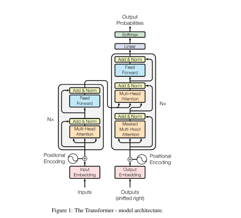
Here, the encoder maps an input sequence representations $(x_{1}, x_{2}, ...., x_{n})$ to a sequence of continuous representations $z = (z_{1}, ...., z_{n})$ . Given $z$ , the decoder then generates an output sequence $(y_{1}, .... y_{n})$ of symbols one element at a time. At each step the model is auto-regressive, consuming the previously generated symbols as additional input when generating the next.

Encoder and Decoder Stacks

The encoder is composed of a stack of $N = 6$ identical layers. Each layer has two sub-layers. The first is a multi-head self attention mechanism, and the second is a simple, position wise fully connected feed forward network.

We employ residual connection around each of the two sub-layers, followed by layer-normalization. That is, output of each sub-layer is

LayerNorm(x + Sublayer(x))

To facilitate the residual connections, all sub-layers in the model, as well as the embedding layers, produce outputs of dimensions $d_{m o d e l} = 512$ .

The decoder is also composed of a stack of $N = 6$ identical layers. In addition to the two sub-layers in each encoder layer, the decoder inserts a third sub-layer, which performs multi-head attention over the output of the encoder stack. Here also we employ residual connections around each sub-layer followed by layer normalization.

We also modify the self-attention sub-layer in the decoder stack to prevent positions from attending to subsequent positions.

Attention

An attention function takes a query, a set a key-value pairs, and produces an output. All of these are vectors. The output is a weighted sum of the values, where the weight given to each value comes from how well the query matches the corresponding key (a compatibility score).

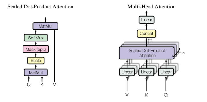
We think of it like a soft lookup table. You have a query (“what am I looking for?”), a bunch of keys (“what does each item represent?”), and values (“the actual content of each item”). Instead of picking one exact match, we compute how similar the query is to every key, turn those similarities into weights, and blend all the values together according to there weights.

This is the specific compatibility function we use. Given queries and keys of dimension $d_{k}$ , the value of the dimension $d_{v}$ :

Attention(O,K,V) = softmax (\frac{Q K ^{T}}{d _{k}}) V

MatMul (Q, K) : Dot product of the query with every key. Raw similarity scores.
Scale : Divide by $d_{k}$
Mask (optional) : Used in the decoder to block attending to future positions.
SoftMax : Converts scores into a probability distribution
MatMul with V : Weighted sum of the value vectors using those probabilities.

Dividing by $d_{k}$ keeps the variance around 1 regardless of dimension, keeping softmax in a well-behaved region.

Instead of doing attention once with full $d_{m o d e l}$ dimensional $Q, K, V$ , we linearly project $Q$ , $K, V$ into $h$ different lower-dimensional sub-spaces, run scaled dot-product attention on each of these projections in parallel, then concatenate all the outputs and project once more.

MultiHead(Q, K, V) = Concat (head_{1}, ...., head_{h})) W^{o}

head_{i} = Attention (Q W_{i}^{Q}, K W_{i}^{K}, V W_{i}^{V})

Multiple head lets the model attend to different representation subspaces at different positions simultaneously. One head might learn to track syntactic dependencies, another might track co-reference, etc.

In this paper $h = 8$ heads, and $d_{k} = d_{v} = d_{m o d e l} / h = 64$ .

This table below shows the complexity for each layer type :

Layer Type	Complexity/Layer	Sequential Ops	Max Path length
Self - Attention	$O (n^{2} . d)$	$O (1)$	$O (1)$
Recurrent	$O (n . d^{2})$	$O (n)$	$O (n)$
Convolutional	$O (k . n . d)$	$O (1)$	$O (l o g_{k} (n))$
Self-Attention (restricted)	$O (r . n . d)$	$O (1)$	$O (n / r)$

Self-attention connects any two positions in one step but pays $O (n^{2})$ cost since it computes pairwise interaction between all positions.

Three ways attention is used in the Transformer

Encoder-decoder attention : Queries come from the decoder, keys/values come from the encoder’s output. This lets every decoder position attend over the entire input sequence - this is the classic seq2seq attention mechanism.
Encoder self-attention : $Q, K, V$ all come from the same place i.e. the previous encoder layer. Every position can attend to every position in the input.
Decoder self-attention (masked) : Same idea, but positions can only attend to earlier positions and itself, not future ones. This preserves the auto-regressive property.

Position-wise Feed-Forward Networks

Each encoder/decoder layer, in addition to attention, has a small feed forward network applied identically and independently to each position. This consists of two linear transformations with a $ReLU$ activation in between :

FEN(x) = max (O, x W_{1} + b_{1}) W_{2} + b_{2}

This is just two linear layers with a $ReLU$ in between. Input/output dimension is $d_{m o d e l} = 512$ , and the linear hidden layer is much wider $d_{f f} = 2048$ .

Embeddings and Softmax

Standard learned embeddings convert input/output tokens into $d_{m o d e l}$ dimensional vectors and a learned linear + softmax converts decoder output back into next-token probabilities.

Positional Encoding

Since there is no recurrence or convolution, the model has no inherent notion of token order. Self-attention treats the sequence like a bag/set. So we inject explicit position information by adding encoding vector to each input embedding, with the same dimension $d_{m o d e l}$ so they can be summed.

In this paper, we use sine and cosine functions of different frequencies :

P E_{(p os, 2 i)} = s in (p os /1000 0^{2 i / d_{m o d e l}})

P E_{(p os, 2 i + 1)} = cos (p os /1000 0^{2 i / d_{m o d e l}})

where $p os$ is the position and $i$ is the dimension. That is, each dimension of the positional encoding corresponds to a sinusoid. The wavelengths form a geometric progression from $2 π$ to $10000.2 π$ .

Digital Garden

Explorer